The p value and the base rate fallacy

You’ve already seen that p values are hard to interpret. Getting a statistically insignificant result doesn’t mean there’s no difference. What about getting a significant result?

Let’s try an example. Suppose I am testing a hundred potential cancer medications. Only ten of these drugs actually work, but I don’t know which; I must perform experiments to find them. In these experiments, I’ll look for \(p<0.05\) gains over a placebo, demonstrating that the drug has a significant benefit.

To illustrate, each square in this grid represents one drug. The blue squares are the drugs that work:

As we saw, most trials can’t perfectly detect every good medication. We’ll assume my tests have a statistical power of 0.8. Of the ten good drugs, I will correctly detect around eight of them, shown in purple:

Of the ninety ineffectual drugs, I will conclude that about 5 have significant effects. Why? Remember that p values are calculated under the assumption of no effect, so \(p = 0.05\) means a 5% chance of falsely concluding that an ineffectual drug works.

So I perform my experiments and conclude there are 13 working drugs: 8 good drugs and 5 I’ve included erroneously, shown in red:

The chance of any given “working” drug being truly effectual is only 62%. If I were to randomly select a drug out of the lot of 100, run it through my tests, and discover a \(p < 0.05\) statistically significant benefit, there is only a 62% chance that the drug is actually effective. In statistical terms, my false discovery rate – the fraction of statistically significant results which are really false positives – is 38%.

Because the base rate of effective cancer drugs is so low – only 10% of our hundred trial drugs actually work – most of the tested drugs do not work, and we have many opportunities for false positives. If I had the bad fortune of possessing a truckload of completely ineffective medicines, giving a base rate of 0%, there is a 0% chance that any statistically significant result is true. Nevertheless, I will get a \(p < 0.05\) result for 5% of the drugs in the truck.

You often hear people quoting p values as a sign that error is unlikely. “There’s only a 1 in 10,000 chance this result arose as a statistical fluke,” they say, because they got \(p = 0.0001\). No! This ignores the base rate, and is called the base rate fallacy. Remember how p values are defined:

The P value is defined as the probability, under the assumption of no effect or no difference (the null hypothesis), of obtaining a result equal to or more extreme than what was actually observed.

A p value is calculated under the assumption that the medication does not work and tells us the probability of obtaining the data we did, or data more extreme than it. It does not tell us the chance the medication is effective.

When someone uses their p values to say they’re probably right, remember this. Their study’s probability of error is almost certainly much higher. In fields where most tested hypotheses are false, like early drug trials (most early drugs don’t make it through trials), it’s likely that most “statistically significant” results with \(p < 0.05\) are actually flukes.

One good example is medical diagnostic tests.

The base rate fallacy in medical testing

There has been some controversy over the use of mammograms in screening breast cancer. Some argue that the dangers of false positive results, such as unnecessary biopsies, surgery and chemotherapy, outweigh the benefits of early cancer detection. This is a statistical question. Let’s evaluate it.

Suppose 0.8% of women who get mammograms have breast cancer. In 90% of women with breast cancer, the mammogram will correctly detect it. (That’s the statistical power of the test. This is an estimate, since it’s hard to tell how many cancers are missed if we don’t know they’re there.) However, among women with no breast cancer at all, about 7% will get a positive reading on the mammogram, leading to further tests and biopsies and so on. If you get a positive mammogram result, what are the chances you have breast cancer?

Ignoring the chance that you, the reader, are male,[1] the answer is 9%.³⁵

Despite the test only giving false positives for 7% of cancer-free women, analogous to testing for \(p < 0.07\), 91% of positive tests are false positives.

How did I calculate this? It’s the same method as the cancer drug example. Imagine 1,000 randomly selected women who choose to get mammograms. Eight of them (0.8%) have breast cancer. The mammogram correctly detects 90% of breast cancer cases, so about seven of the eight women will have their cancer discovered. However, there are 992 women without breast cancer, and 7% will get a false positive reading on their mammograms, giving us 70 women incorrectly told they have cancer.

In total, we have 77 women with positive mammograms, 7 of whom actually have breast cancer. Only 9% of women with positive mammograms have breast cancer.

If you administer questions like this one to statistics students and scientific methodology instructors, more than a third fail.³⁵ If you ask doctors, two thirds fail.¹⁰ They erroneously conclude that a \(p < 0.05\) result implies a 95% chance that the result is true – but as you can see in these examples, the likelihood of a positive result being true depends on what proportion of hypotheses tested are true. And we are very fortunate that only a small proportion of women have breast cancer at any given time.

Examine introductory statistical textbooks and you will often find the same error. P values are counterintuitive, and the base rate fallacy is everywhere.

Taking up arms against the base rate fallacy

You don’t have to be performing advanced cancer research or early cancer screenings to run into the base rate fallacy. What if you’re doing social research? You’d like to survey Americans to find out how often they use guns in self-defense. Gun control arguments, after all, center on the right to self-defense, so it’s important to determine whether guns are commonly used for defense and whether that use outweighs the downsides, such as homicides.

One way to gather this data would be through a survey. You could ask a representative sample of Americans whether they own guns and, if so, whether they’ve used the guns to defend their homes in burglaries or defend themselves from being mugged. You could compare these numbers to law enforcement statistics of gun use in homicides and make an informed decision about whether the benefits outweigh the downsides.

Such surveys have been done, with interesting results. One 1992 telephone survey estimated that American civilians use guns in self-defense up to 2.5 million times every year – that is, about 1% of American adults have defended themselves with firearms. Now, 34% of these cases were in burglaries, giving us 845,000 burglaries stymied by gun owners. But in 1992, there were only 1.3 million burglaries committed while someone was at home. Two thirds of these occurred while the homeowners were asleep and were discovered only after the burglar had left. That leaves 430,000 burglaries involving homeowners who were at home and awake to confront the burglar – 845,000 of which, we are led to believe, were stymied by gun-toting residents.²⁸

Whoops.

What happened? Why did the survey overestimate the use of guns in self-defense? Well, for the same reason that mammograms overestimate the incidence of breast cancer: there are far more opportunities for false positives than false negatives. If 99.9% of people have never used a gun in self-defense, but 1% of those people will answer “yes” to any question for fun, and 1% want to look manlier, and 1% misunderstand the question, then you’ll end up vastly overestimating the use of guns in self-defense.

What about false negatives? Could this effect be balanced by people who say “no” even though they gunned down a mugger last week? No. If very few people genuinely use a gun in self-defense, then there are very few opportunities for false negatives. They’re overwhelmed by the false positives.

This is exactly analogous to the cancer drug example earlier. Here, p is the probability that someone will falsely claim they’ve used a gun in self-defense. Even if p is small, your final answer will be wildly wrong.

To lower p, criminologists make use of more detailed surveys. The National Crime Victimization surveys, for instance, use detailed sit-down interviews with researchers where respondents are asked for details about crimes and their use of guns in self-defense. With far greater detail in the survey, researchers can better judge whether the incident meets their criteria for self-defense. The results are far smaller – something like 65,000 incidents per year, not millions. There’s a chance that survey respondents underreport such incidents, but a much smaller chance of massive overestimation.

If at first you don’t succeed, try, try again

The base rate fallacy shows us that false positives are much more likely than you’d expect from a \(p < 0.05\) criterion for significance. Most modern research doesn’t make one significance test, however; modern studies compare the effects of a variety of factors, seeking to find those with the most significant effects.

For example, imagine testing whether jelly beans cause acne by testing the effect of every single jelly bean color on acne:

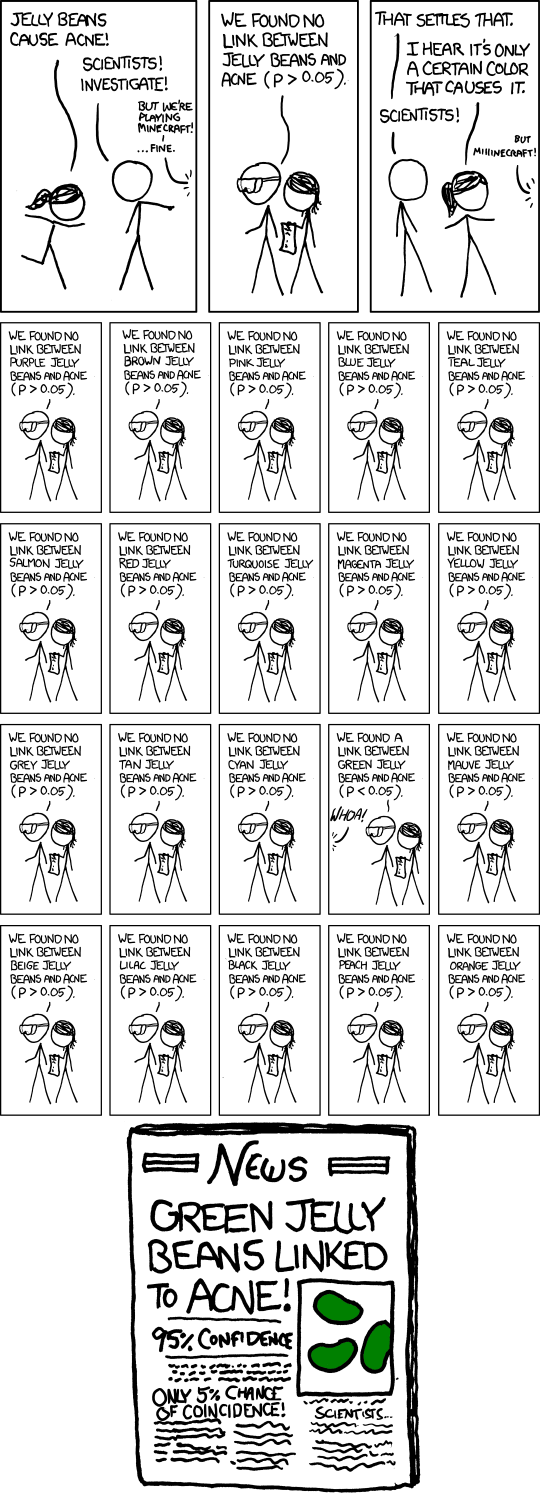
Cartoon from xkcd, by Randall Munroe. http://xkcd.com/882/

As you can see, making multiple comparisons means multiple chances for a false positive. For example, if I test 20 jelly bean flavors which do not cause acne at all, and look for a correlation at \(p < 0.05\) significance, I have a 64% chance of a false positive result.⁵⁴ If I test 45 materials, the chance of false positive is as high as 90%.

It’s easy to make multiple comparisons, and it doesn’t have to be as obvious as testing twenty potential medicines. Track the symptoms of a dozen patients for a dozen weeks and test for significant benefits during any of those weeks: bam, that’s twelve comparisons. Check for the occurrence of twenty-three potential dangerous side effects: alas, you have sinned. Send out a ten-page survey asking about nuclear power plant proximity, milk consumption, age, number of male cousins, favorite pizza topping, current sock color, and a few dozen other factors for good measure, and you’ll find that something causes cancer. Ask enough questions and it’s inevitable.

A survey of medical trials in the 1980s found that the average trial made 30 therapeutic comparisons. In more than half of the trials, the researchers had made so many comparisons that a false positive was highly likely, and the statistically significant results they did report were cast into doubt: they may have found a statistically significant effect, but it could just have easily been a false positive.⁵⁴

There exist techniques to correct for multiple comparisons. For example, the Bonferroni correction method says that if you make \(n\) comparisons in the trial, your criterion for significance should be \(p < 0.05/n\). This lowers the chances of a false positive to what you’d see from making only one comparison at \(p < 0.05\). However, as you can imagine, this reduces statistical power, since you’re demanding much stronger correlations before you conclude they’re statistically significant. It’s a difficult tradeoff, and tragically few papers even consider it.

Red herrings in brain imaging

Neuroscientists do massive numbers of comparisons regularly. They often perform fMRI studies, where a three-dimensional image of the brain is taken before and after the subject performs some task. The images show blood flow in the brain, revealing which parts of the brain are most active when a person performs different tasks.

But how do you decide which regions of the brain are active during the task? A simple method is to divide the brain image into small cubes called voxels. A voxel in the “before” image is compared to the voxel in the “after” image, and if the difference in blood flow is significant, you conclude that part of the brain was involved in the task. Trouble is, there are thousands of voxels to compare and many opportunities for false positives.

One study, for instance, tested the effects of an “open-ended mentalizing task” on participants. Subjects were shown “a series of photographs depicting human individuals in social situations with a specified emotional valence,” and asked to “determine what emotion the individual in the photo must have been experiencing.” You can imagine how various emotional and logical centers of the brain would light up during this test.

The data was analyzed, and certain brain regions found to change activity during the task. Comparison of images made before and after the mentalizing task showed a \(p = 0.001\) difference in a \(81 \text{mm}^3\) cluster in the brain.

The study participants? Not college undergraduates paid $10 for their time, as is usual. No, the test subject was one 3.8-pound Atlantic salmon, which “was not alive at the time of scanning.”⁸

Of course, most neuroscience studies are more sophisticated than this; there are methods of looking for clusters of voxels which all change together, along with techniques for controlling the rate of false positives even when thousands of statistical tests are made. These methods are now widespread in the neuroscience literature, and few papers make such simple errors as I described. Unfortunately, almost every paper tackles the problem differently; a review of 241 fMRI studies found that they performed 223 unique analysis strategies, which, as we will discuss later, gives the researchers great flexibility to achieve statistically significant results.¹³

Controlling the false discovery rate

I mentioned earlier that techniques exist to correct for multiple comparisons. The Bonferroni procedure, for instance, says that you can get the right false positive rate by looking for \(p < 0.05/n\), where \(n\) is the number of statistical tests you’re performing. If you perform a study which makes twenty comparisons, you can use a threshold of \(p < 0.0025\) to be assured that there is only a 5% chance you will falsely decide a nonexistent effect is statistically significant.

This has drawbacks. By lowering the p threshold required to declare a result statistically significant, you decrease your statistical power greatly, and fail to detect true effects as well as false ones. There are more sophisticated procedures than the Bonferroni correction which take advantage of certain statistical properties of the problem to improve the statistical power, but they are not magic solutions.

Worse, they don’t spare you from the base rate fallacy. You can still be misled by your p threshold and falsely claim there’s “only a 5% chance I’m wrong” – you just eliminate some of the false positives. A scientist is more interested in the false discovery rate: what fraction of my statistically significant results are false positives? Is there a statistical test that will let me control this fraction?

For many years the answer was simply “no.” As you saw in the section on the base rate fallacy, we can compute the false discovery rate if we make an assumption about how many of our tested hypotheses are true – but we’d rather find that out from the data, rather than guessing.

In 1995, Benjamini and Hochberg provided a better answer. They devised an exceptionally simple procedure which tells you which p values to consider statistically significant. I’ve been saving you from mathematical details so far, but to illustrate just how simple the procedure is, here it is:

1. Perform your statistical tests and get the p value for each. Make a list and sort it in ascending order.
2. Choose a false-discovery rate and call it q. Call the number of statistical tests m.
3. Find the largest p value such that \(p \leq i q/m\), where i is the p value’s place in the sorted list.
4. Call that p value and all smaller than it statistically significant.

You’re done! The procedure guarantees that out of all statistically significant results, no more than q percent will be false positives.⁷

The Benjamini-Hochberg procedure is fast and effective, and it has been widely adopted by statisticians and scientists in certain fields. It usually provides better statistical power than the Bonferroni correction and friends while giving more intuitive results. It can be applied in many different situations, and variations on the procedure provide better statistical power when testing certain kinds of data.

Of course, it’s not perfect. In certain strange situations, the Benjamini-Hochberg procedure gives silly results, and it has been mathematically shown that it is always possible to beat it in controlling the false discovery rate. But it’s a start, and it’s much better than nothing.

[1]	Interestingly, being male doesn’t exclude you from getting breast cancer; it just makes it exceedingly unlikely.